Data Analysis

Tasks

1. Use the cleaned dataset (.RData)
2. Clearly state your research questions
3. Answer each question with analysis, step by step
4. Explain what you’re doing and why (use comments in your R code)
5. Briefly summarize the key finding(s) after each question

Preliminary Set-Up

Load the packages

library(tidyverse)

── Attaching core tidyverse packages ──────────────────────── tidyverse 2.0.0 ──
✔ dplyr     1.1.4     ✔ readr     2.1.5
✔ forcats   1.0.0     ✔ stringr   1.5.1
✔ ggplot2   3.5.2     ✔ tibble    3.3.0
✔ lubridate 1.9.4     ✔ tidyr     1.3.1
✔ purrr     1.1.0     
── Conflicts ────────────────────────────────────────── tidyverse_conflicts() ──
✖ dplyr::filter() masks stats::filter()
✖ dplyr::lag()    masks stats::lag()
ℹ Use the conflicted package (<http://conflicted.r-lib.org/>) to force all conflicts to become errors

library(sf)

Linking to GEOS 3.13.0, GDAL 3.8.5, PROJ 9.5.1; sf_use_s2() is TRUE

library(dplyr)
library(ggplot2)
library(viridis)

Loading required package: viridisLite

library(gridExtra)

Attaching package: 'gridExtra'

The following object is masked from 'package:dplyr':

    combine

library(patchwork)
library(rnaturalearth)
library(rnaturalearthdata)

Attaching package: 'rnaturalearthdata'

The following object is masked from 'package:rnaturalearth':

    countries110

Load cleaned datasets

load("gdp_clean.RData")
load("PlasticWasteCountry_clean.RData")
load("PlasticWasteRegion_clean.RData") 

Research Questions

1. How much plastic waste has been generated per person/kg/day in each country in East and Southeast Asia?
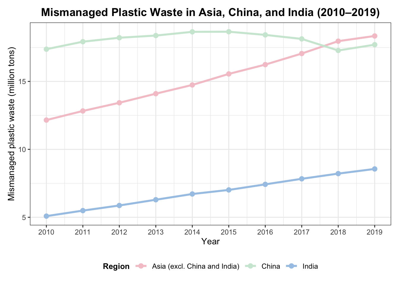
2. Which countries in East & Southeast Asia produced the highest levels of plastic waste, and how did the pattern change from 2010 to 2019?
3. To what extent is there a correlation between a country’s GDP per capita and its plastic waste emission?

How much plastic waste has been generated per person/kg/day in each country in East and Southeast Asia?

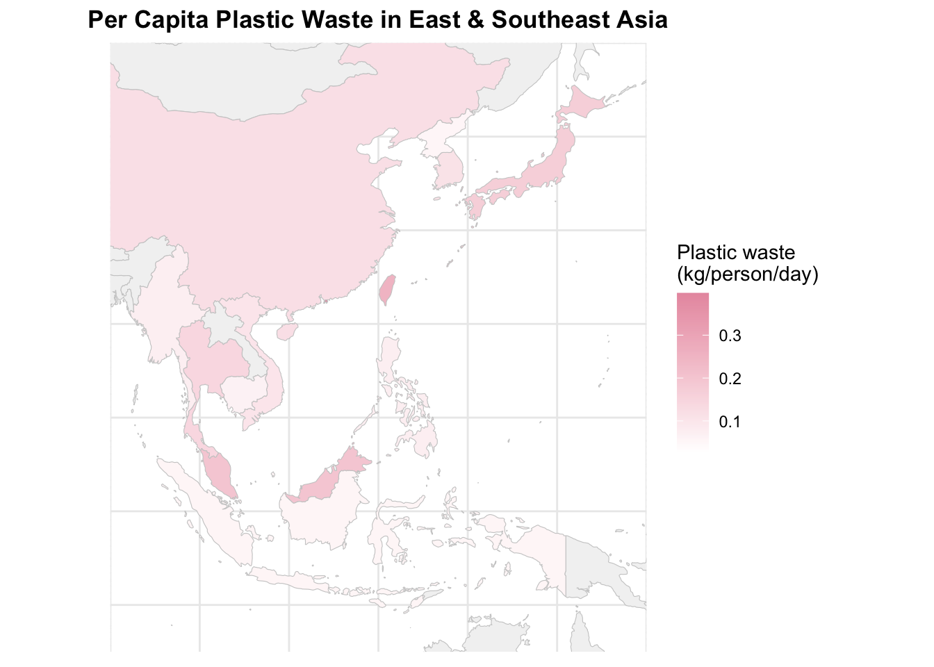
1. Map - Geographical pattern of plastic waste

# Step 1: Get Asia map
world <- ne_countries(scale = "medium", returnclass = "sf")

# Step 3: Prepare plastic waste data for mapping and join them to the map
plastic_map <- PlasticWasteCountry3 |>
  rename(
    iso_a3 = iso_code,
    waste_pc = waste_kg_day
  )
world_plastic_2010 <- world |>
  left_join(plastic_map, by = c("iso_a3"))

# Step 4: Make a plastic waste map
map_plastic <- ggplot(world_plastic_2010) +
  geom_sf(aes(fill = waste_pc), color = "gray80", size = 0.1) +
  scale_fill_gradient(low = "#FFFFFF", high = "#E89AAE", na.value = "gray95") +
  coord_sf(xlim = c(90, 150), ylim = c(-15, 50), expand = FALSE) +
  labs(title = "Per Capita Plastic Waste in East & Southeast Asia",
    fill = "Plastic waste\n(kg/person/day)") +
  theme_minimal() +
  theme(
    plot.title = element_text(face = "bold", hjust = 0.5),
    axis.title = element_blank(),
    axis.text = element_blank(),
    axis.ticks = element_blank()
  )

map_plastic

Key findings: Higher plastic waste emissions are observed in high-income countries such as Singapore and Japan, followed by China and South Korea. A large share of plastic waste emissions is found in Taiwan (at least according to data from Our World in Data).

Which countries in East & Southeast Asia produced the highest levels of plastic waste, and how did the pattern change from 2010 to 2019?

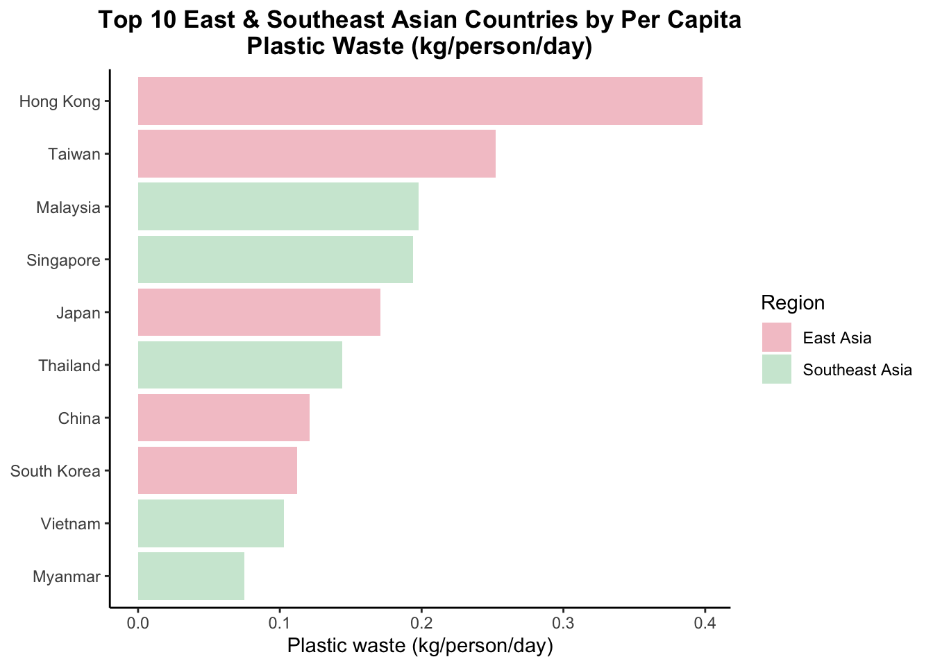
2.1 Bar chart – Top 10 plastic waste–producing countries (per capita)

# Step 1: Rank by waste_kg_day
rq1 <- PlasticWasteCountry3 |>
  arrange(desc(waste_kg_day)) |>
  mutate(
    country = fct_reorder(country, waste_kg_day)
  )

# Step 2: Take the top 10 countries
rq1_top10 <- rq1 |>
  slice_head(n = 10)
rq1_top10

# A tibble: 10 × 5
   country     iso_code  year waste_kg_day region_group  
   <fct>       <chr>    <dbl>        <dbl> <chr>         
 1 Hong Kong   HKG       2010        0.398 East Asia     
 2 Taiwan      TWN       2010        0.252 East Asia     
 3 Malaysia    MYS       2010        0.198 Southeast Asia
 4 Singapore   SGP       2010        0.194 Southeast Asia
 5 Japan       JPN       2010        0.171 East Asia     
 6 Thailand    THA       2010        0.144 Southeast Asia
 7 China       CHN       2010        0.121 East Asia     
 8 South Korea KOR       2010        0.112 East Asia     
 9 Vietnam     VNM       2010        0.103 Southeast Asia
10 Myanmar     MMR       2010        0.075 Southeast Asia

Key findings: Hong Kong has the highest plastic waste produced per day, followed by Taiwan and Malaysia. Top 10 countries’ waste kilogram ranges from 0.398 to 0.075.

# Step 3: Plot bar chart of top 10 waste-producing countries
bar_top10 <- ggplot(rq1_top10, aes(x = country, y = waste_kg_day, fill = region_group)) +
  geom_col() +
  coord_flip() +
  scale_fill_manual(values = c("East Asia" = "#F4C7CE", "Southeast Asia" = "#CFE8D6")) +
  labs(title = "Top 10 East & Southeast Asian Countries by Per Capita\nPlastic Waste (kg/person/day)",
    x = "Country",
    y = "Plastic waste (kg/person/day)",
    fill = "Region") +
  theme_classic() +
  theme(
    plot.title = element_text(face = "bold", hjust = 0.5),
    axis.title.y = element_blank()
  )

bar_top10

Key findings: Hong Kong, Taiwan, and Malaysia appear among the highest per capita plastic waste producers in East Asia and Southeast Asia. The number of East Asian and South Asian countries in the top 10 plastic waste producers list was roughly equal, with East Asian countries slightly taking the lead.

2.2 Line chart – Plastic waste trends for Asia (excl. China & India), China, and India (2010–2019)

region_series <- PlasticWasteRegion3 |>
  filter(year >= 2010, year <= 2019) |>
  filter(country %in% c("Asia (excl. China and India)", "China", "India"))

# Ensure regions appear in a consistent order for clearer interpretation
line_regions <- region_series |>
  mutate(
    country = factor(country, levels = c("Asia (excl. China and India)", "China", "India"))) |>
# Draw the line plot
  ggplot(aes(x = year, y = mismanaged_tons / 1e6, color = country)) +
  geom_line(size = 1.2) +
  geom_point(size = 2.5) +
  scale_x_continuous(breaks = 2010:2019) +
  scale_y_continuous(labels = scales::comma) +
  scale_color_manual(
    values = c("Asia (excl. China and India)" = "#F4C7CE", "China" = "#CFE8D6", "India" = "#A7C7E7")) +
  labs(title = "Mismanaged Plastic Waste in Asia, China, and India (2010–2019)",
    x = "Year",
    y = "Mismanaged plastic waste (million tons)",
    color = "Region") +
  theme_bw() +
  theme(
    plot.title = element_text(face = "bold", hjust = 0.5, size = 14),
    axis.title = element_text(size = 11),
    axis.text = element_text(size = 9),
    legend.position = "bottom",
    legend.title = element_text(size = 10, face = "bold"),
    legend.text = element_text(size = 9),
    plot.margin = margin(10, 10, 10, 10)  # adds breathing room
  )

Warning: Using `size` aesthetic for lines was deprecated in ggplot2 3.4.0.
ℹ Please use `linewidth` instead.

line_regions

Key findings: Asia (excluding China and India) ’s plastic waste emissions increased steadily each year, while China’s declined from 2015 to 2018 after peaking around 2014 and 2015. India also shows a clear upward trajectory over the decade, though its total plastic waste emissions remain significantly lower than those of China and Asia.

To what extent is there a correlation between a country’s GDP per capita and its plastic waste emission?

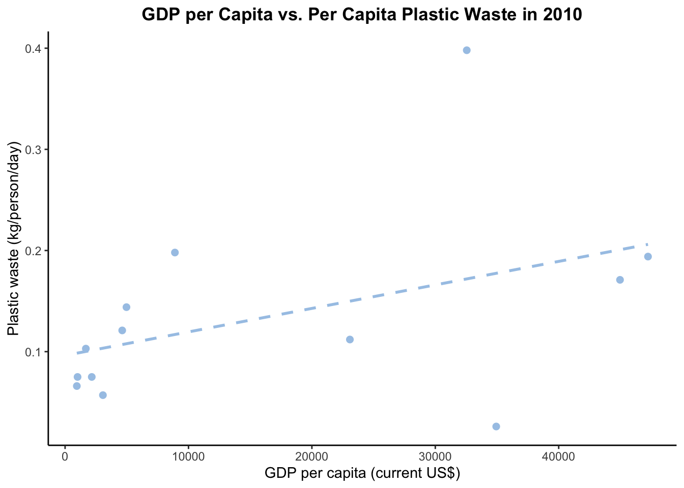
3. Scatter plot - Correlation between GDP per capita and plastic waste

# Step 1: Filter GDP to 2010
gdp_2010 <- gdp_asia |>
  filter(year == 2010)

# Step 2: Merge by iso_code since its safer than country name
gdp_plastic_2010 <- PlasticWasteCountry3 |>
  inner_join(gdp_2010, by = c("iso_code" = "country_code"))
gdp_plastic_2010

# A tibble: 13 × 10
   country.x  iso_code year.x waste_kg_day region_group.x country.y country_name
   <chr>      <chr>     <dbl>        <dbl> <chr>          <chr>     <chr>       
 1 Brunei     BRN        2010        0.026 Southeast Asia Brunei    Brunei Daru…
 2 Cambodia   KHM        2010        0.066 Southeast Asia Cambodia  Cambodia    
 3 China      CHN        2010        0.121 East Asia      China     China       
 4 Hong Kong  HKG        2010        0.398 East Asia      Hong Kong Hong Kong S…
 5 Indonesia  IDN        2010        0.057 Southeast Asia Indonesia Indonesia   
 6 Japan      JPN        2010        0.171 East Asia      Japan     Japan       
 7 Malaysia   MYS        2010        0.198 Southeast Asia Malaysia  Malaysia    
 8 Myanmar    MMR        2010        0.075 Southeast Asia Myanmar   Myanmar     
 9 Philippin… PHL        2010        0.075 Southeast Asia Philippi… Philippines 
10 Singapore  SGP        2010        0.194 Southeast Asia Singapore Singapore   
11 South Kor… KOR        2010        0.112 East Asia      South Ko… Korea, Rep. 
12 Thailand   THA        2010        0.144 Southeast Asia Thailand  Thailand    
13 Vietnam    VNM        2010        0.103 Southeast Asia Vietnam   Viet Nam    
# ℹ 3 more variables: year.y <dbl>, gdp_per_capita <dbl>, region_group.y <chr>

# Step 3: Create the scatter plot and draw a trend line
scatter_gdp <- ggplot(gdp_plastic_2010, aes(x = gdp_per_capita, y = waste_kg_day)) +
  geom_point(size = 2, color = "#A7C7E7") +
  geom_smooth(method = "lm", se = FALSE, color = "#A7C7E7", linetype = "dashed") +
  scale_color_viridis_d(option = "magma") +
  labs(title = "GDP per Capita vs. Per Capita Plastic Waste in 2010",
    x = "GDP per capita (current US$)",
    y = "Plastic waste (kg/person/day)",
    color = "Region") +
  theme_classic() +
  theme(plot.title = element_text(face = "bold", hjust = 0.5))

scatter_gdp

`geom_smooth()` using formula = 'y ~ x'

Key findings: Overall, a country’s plastic waste emission (kg/person/day) shows a positive correlation with its GDP per capita. However, there are still some outliers, such as Hong Kong, with the highest level of plastic waste but a moderately high GDP.

Saving the Graphs

# 1. - Map - Geographical pattern of plastic waste
ggsave("photos/map_plastic.png", plot = map_plastic, width = 10, height = 6, dpi = 300)

# 2.1 Bar chart – Top 10 plastic waste–producing countries (per capita)
ggsave("photos/bar_top10.png", plot = bar_top10, width = 10, height = 6, dpi = 300)

# 2.2 Line chart – Plastic waste trends for Asia (excl. China & India), China, and India (2010–2019)
ggsave("photos/line_regions.png", plot = line_regions, width = 10, height = 6, dpi = 300)

# 3. Scatter plot - Correlation between GDP per capita and plastic waste
ggsave("photos/scatter_gdp.png", plot = scatter_gdp, width = 10, height = 6, dpi = 300)

`geom_smooth()` using formula = 'y ~ x'